Binding energy calculation
Download Tutorial Package
To download the tutorial package, click on this link. This package contains required file for the tutorial.
Untar this package by following command:
tar -zxvf tutorial.tar.gz
cd tutorial
cd 1EBZ
This directory contains topology-parameter (tpr),
atom-index (ndx), and trajectory (xtc) files of a HIV-1 protease inhibitor complex.
Calculation of three energy components
The binding energy consists of three energetic terms,
potential energy in vacuum,
polar-solvation energy and
non-polar solvation energy.
These energetic terms could be calculated in either three or one step.
Three steps calculation
1. Calculation of potential energy in Vacuum
Execute the following command:
g_mmpbsa run -f 1EBZ.xtc -s 1EBZ.tpr -n 1EBZ.ndx -pdie 2 -decomp -unit1 Protein -unit2 BEC
Here we are selecting Protein as unit-1 and BEC, which is a ligand, as unit-2. The binding
energy will be calculated between the protein and ligand.
Two files energy_MM.xvg and contrib_MM.dat are generated as outputs.
Both files could be generated with different name by
-mm filename1.xvg and -mmcon filename2.dat.
energy_MM.xvg file contains van der Waals, electrostatic interactions, and net non-bonded potential
energy between the protein and inhibitor.
contrib_MM.dat contains contribution of each residue to the calculated net
non-bonded interaction energy.
2. Calculation of polar solvation energy
To calculate the polar solvation energy, an input file (e.g. tutorial/polar.mdp) is required. This file contains input parameters that are used in the calculation of polar solvation energy.
Execute the following command:
g_mmpbsa run -f 1EBZ.xtc -s 1EBZ.tpr -n 1EBZ.ndx -i ../polar.mdp -nomme -pbsa \
             -decomp -unit1 Protein -unit2 BEC -pol polar.xvg -pcon contrib_pol.dat
Two files polar.xvg and contrib_pol.dat are generated as outputs.
Both files could be generated with different name by -pol filename1.xvg
and -pcon filename2.dat.
polar.xvg contains polar solvation energies for unbound protein, unbound inhibitor
and protein-inhibitor complex.
contrib_pol.dat contains contribution of each residue to the calculated net polar
solvation energy.
3. Calculation of non-polar solvation energy
To calculate the non-polar solvation energy, an input file (e.g. tutorial/apolar_sasa.mdp) is required. This file contains parameters that are used in the calculation of non-polar solvation energy.
There are several type of non-polar models that are discussed in the g_mmpbsa publication. Here, SASA-only and SAV-only model are used for which input parameter files are provided.
Warning
Now WCA model is removed from the g_mmpbsa package.
For SASA-only model:
Execute the following command:
g_mmpbsa run -f 1EBZ.xtc -s 1EBZ.tpr -n 1EBZ.ndx -i ../apolar_sasa.mdp -nomme -pbsa -decomp \
             -unit1 Protein -unit2 BEC -apol sasa.xvg -apcon sasa_contrib.dat
Two files sasa.xvg and sasa_contrib.dat are generated as outputs.
sasa.xvg contains non-polar solvation energy for unbound protein,
unbound inhibitor and protein-inhibtor complex. sasa_contrib.dat
contains contribution of each residue to the calculated net polar-solvation energy.
For SAV-only model:
Execute the following command:
g_mmpbsa run -f 1EBZ.xtc -s 1EBZ.tpr -n 1EBZ.ndx -i ../apolar_sav.mdp -nomme -pbsa -decomp \
             -unit1 Protein -unit2 BEC -apol sav.xvg -apcon sav_contrib.dat`
Two files sav.xvg and sav_contrib.dat are generated as outputs.
sav.xvg contains non-polar solvation energy for unbound protein,
unbound inhibitor and protein-inhibtor complex. sav_contrib.dat
contains contribution of each residue to the calculated net polar-solvation energy.
One step calculation
Execute the following command:
g_mmpbsa run -f 1EBZ.xtc -s 1EBZ.tpr -n 1EBZ.ndx -i ../pbsa.mdp -pdie 2 -pbsa -decomp \
             -unit1 Protein -unit2 BEC -os energy_summary.csv \
             -ores residues_energy_summary.csv -silent
Here we are selecting Protein as unit-1 and BEC, which is a ligand, as unit-2. The binding
energy will be calculated between the protein and ligand.
pbsa.mdp contains input parameters for both polar and SASA-only non-polar solvation energies.
All three energetic terms are calculated by using the above single command and all output files
are generated.
-os energy_summary.csv
It will also calculate average binding energy and standard deviation of all the energy terms
and will be output in CSV format energy_summary.csv file provided with -os option.
This file can be directly opened in MS excel or any other spreadsheet software.
"Energy"             , "Average", "Standard-Deviation",
"vDW"                , -334.587 ,               15.897,
"Electrostatic"      , -318.759 ,               32.401,
"Polar-solvation"    , 313.703  ,               10.426,
"Non-polar-solvation", -30.420  ,                1.016,
"Total"              , -370.062 ,               32.903,
-ores residues_energy_summary.csv
This file contain summary of binding energy contributions (both average and standard deviation) of residues over all frames.
The output file has following rows and columns:
"Residue", "vDW"   , "vdW-stddev", "Elec." , "Elec.-stdev", "polar", "polar-stdev", "apolar", "apolar-stdev", "total" , "total-stdev",
"PRO-1"  , -0.004  ,        0.001, 0.655   ,         0.660, -0.202 ,         0.186, 0.000   ,          0.000, 0.449   ,         0.520,
"GLN-2"  , -0.005  ,        0.000, 0.094   ,         0.074, -0.112 ,         0.060, 0.000   ,          0.000, -0.023  ,         0.032,
"ILE-3"  , -0.018  ,        0.003, -0.083  ,         0.035, 0.101  ,         0.025, 0.000   ,          0.000, -0.000  ,         0.029,
"THR-4"  , -0.014  ,        0.001, -0.013  ,         0.073, 0.004  ,         0.044, 0.000   ,          0.000, -0.022  ,         0.062,
"LEU-5"  , -0.078  ,        0.009, 0.169   ,         0.061, -0.015 ,         0.056, 0.000   ,          0.000, 0.076   ,         0.055,
"TRP-6"  , -0.039  ,        0.005, 0.164   ,         0.056, 0.009  ,         0.025, 0.000   ,          0.000, 0.134   ,         0.052,
"GLN-7"  , -0.068  ,        0.014, -0.211  ,         0.152, 0.238  ,         0.086, 0.000   ,          0.000, -0.040  ,         0.132,
"ARG-8"  , -5.167  ,        1.695, -3.454  ,         4.016, 9.184  ,         4.154, -0.637  ,          0.191, -0.074  ,         3.831,
"PRO-9"  , -0.202  ,        0.041, -0.029  ,         0.120, 0.076  ,         0.072, 0.000   ,          0.000, -0.155  ,         0.122,
"LEU-10" , -0.196  ,        0.057, -0.046  ,         0.061, 0.034  ,         0.027, 0.000   ,          0.000, -0.208  ,         0.077,
.
.
.
Average Binding Energy Calculation
The average binding energies can be directly calculated in one-step method as described above. However, the bootstrap analysis could be used to calculate the average binding energy with standard error.
To calculate average binding energy, execute following command:
g_mmpbsa average -m energy_MM.xvg -p polar.xvg -a apolar.xvg -bs
Three output files full_energy.dat, summary_energy.dat and
summary_energy.csv are obtained. Both summary_energy.dat and summary_energy.csv
contains average and standard deviations of all energetic components
including the binding energy as follows:
#Complex Number:    1
===============
   SUMMARY
===============

 van der Waal energy      =        -334.587   +/-   15.514 kJ/mol

 Electrostattic energy    =        -159.380   +/-   15.810 kJ/mol

 Polar solvation energy   =         313.698   +/-   10.174 kJ/mol

 SASA energy              =         -30.431   +/-    0.996 kJ/mol

 SAV energy               =           0.000   +/-    0.000 kJ/mol

 WCA energy               =           0.000   +/-    0.000 kJ/mol

 Binding energy           =        -210.699   +/-   19.745 kJ/mol

===============
    END
===============
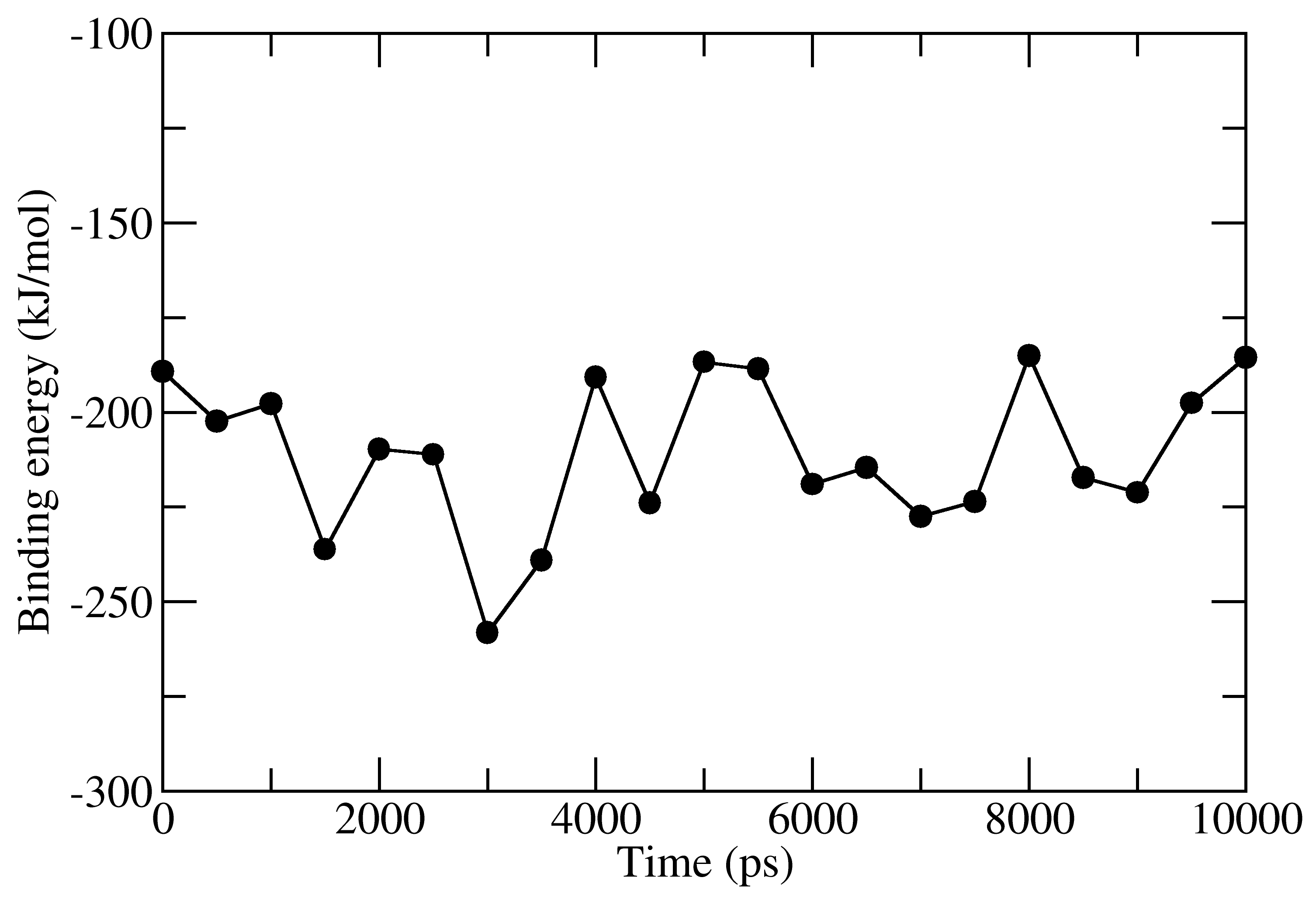
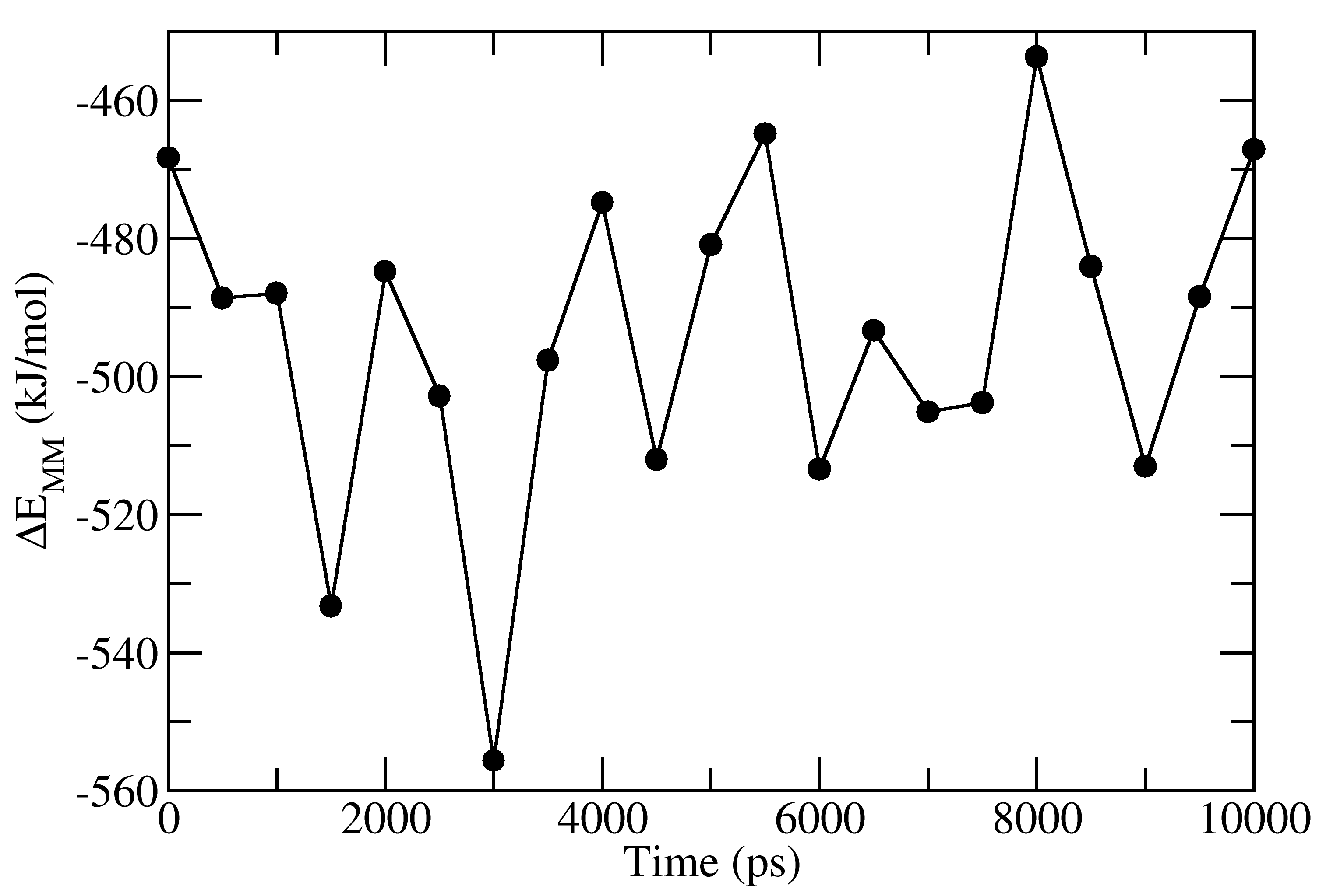
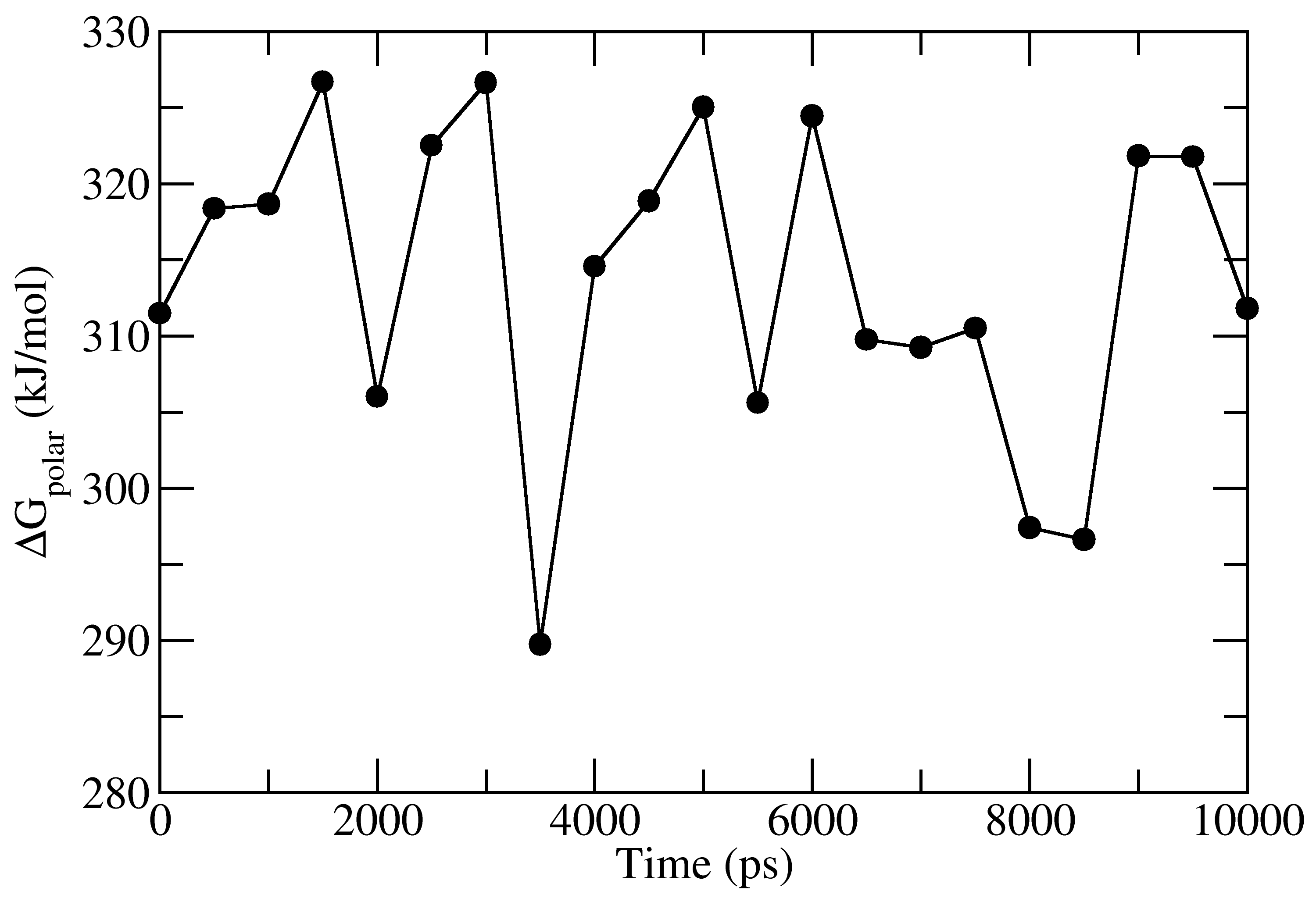
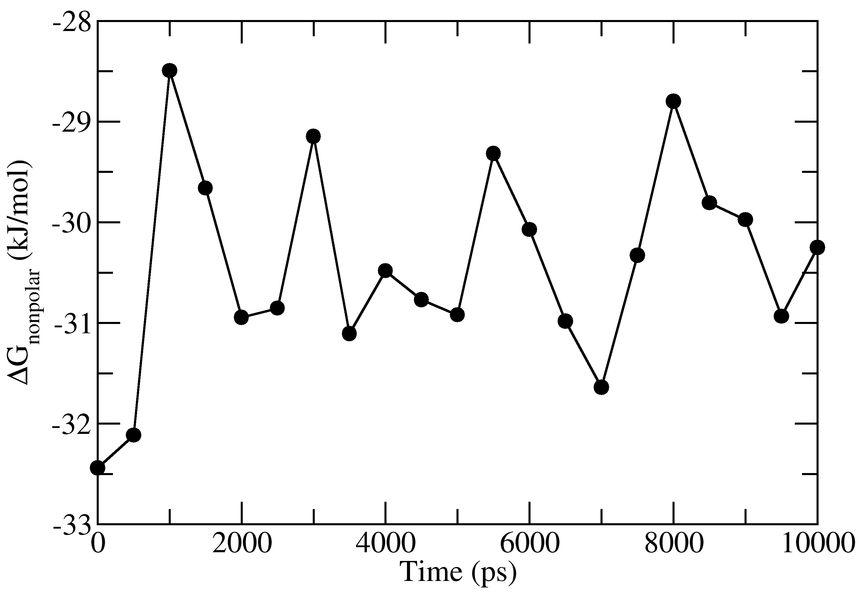
full_energy.dat contains the values of energetic terms as a function of time.
Last four columns contains Δ_E_<sub>MM</sub>, Δ_G_<sub>polar</sub>, Δ_G_<sub>nonpolar</sub> and Δ_G_<sub>binding</sub>
as a function of time. These quantities could be plotted with xmgrace/matplotlib/gnuplot.
The respective four files in xmgrace format (_agr_) are provided in tutorial/1EBZ/output
To calculate average binding energy by using bootstrap analysis, execute following command:
g_mmpbsa run -bs -nbs 2000 -m energy_MM.xvg -p polar.xvg -a apolar.xvg
Again, two output files full_energy.dat and summary_energy.dat are generated as outputs.
full_energy.dat is similar to that of the above one.
However, summary_energy.dat contains average and standard error of all energetic components
including the binding energy.
Average values in summary_energy.dat are slightly different from the above one.
For more details about this method, please follow the g_mmpbsa publication.